library(lifelihood)
#> Loading required package: tidyverse
#> ── Attaching core tidyverse packages ──────────────────────── tidyverse 2.0.0 ──
#> ✔ dplyr     1.2.0     ✔ readr     2.2.0
#> ✔ forcats   1.0.1     ✔ stringr   1.6.0
#> ✔ ggplot2   4.0.2     ✔ tibble    3.3.1
#> ✔ lubridate 1.9.5     ✔ tidyr     1.3.2
#> ✔ purrr     1.2.1
#> ── Conflicts ────────────────────────────────────────── tidyverse_conflicts() ──
#> ✖ dplyr::filter() masks stats::filter()
#> ✖ dplyr::lag()    masks stats::lag()
#> ℹ Use the conflicted package (<http://conflicted.r-lib.org/>) to force all conflicts to become errors
library(tidyverse)

df <- datapierrick |>
  as_tibble() |>
  mutate(
    par = as.factor(par),
    geno = as.factor(geno),
    spore = as.factor(spore),
    block = rep(1:2, each = nrow(datapierrick) / 2)
  )

generate_clutch_vector <- function(N) {
  return(paste(
    "pon",
    rep(c("start", "end", "size"), N),
    rep(1:N, each = 3),
    sep = "_"
  ))
}
clutchs <- generate_clutch_vector(28)

lifelihoodData <- as_lifelihoodData(
  df = df,
  sex = "sex",
  sex_start = "sex_start",
  sex_end = "sex_end",
  maturity_start = "mat_start",
  maturity_end = "mat_end",
  clutchs = clutchs,
  block = "block",
  death_start = "death_start",
  death_end = "death_end",
  covariates = c("par", "spore"),
  model_specs = c("wei", "gam", "lgn")
)Create a lifelihoodData object
Standard errors
By default, lifelihood will not try to fit standard errors. But, you can use the se.fit argument for this purpose:
results <- lifelihood(
  lifelihoodData = lifelihoodData,
  path_config = use_test_config("example_config_se"),
  se.fit = TRUE,
)
#> [1] "/Users/runner/work/_temp/Library/lifelihood/bin/lifelihood-macos /Users/runner/work/Lifelihood/Lifelihood/lifelihood_2826_9893_4331_7519/temp_file_data_lifelihood.txt /Users/runner/work/Lifelihood/Lifelihood/lifelihood_2826_9893_4331_7519/temp_param_range_path.txt 0 25 TRUE 0 FALSE 0 2826 9893 4331 7519 10 20 1000 0.3 NULL 2 2 50 1 1 0.001"
summary(results)
#>
#> === LIFELIHOOD RESULTS ===
#>
#> Sample size: 550
#>
#> --- Model Fit ---
#> Log-likelihood:  -343784.808
#> AIC:             687577.6
#> BIC:             687594.9
#>
#> --- Key Parameters ---
#>
#> Mortality:
#>   expt_death (Intercept)    -1.962 (0.072)
#>   expt_death eff_expt_death_par_1 0.302 (0.078)
#>   expt_death eff_expt_death_par_2 0.254 (0.084)
#>   survival_param2 (Intercept) -0.210 (0.115)
#>
#> --- Convergence ---
#> All parameters within bounds
#>
#> ======================
Now if we have a look at the estimations we have standard errors:
results$effects |> as_tibble()
#> # A tibble: 4 × 6
#>   name                 estimation stderror parameter       kind            event
#>   <chr>                     <dbl>    <dbl> <chr>           <chr>           <chr>
#> 1 int_expt_death           -1.96    0.0724 expt_death      intercept       mort…
#> 2 eff_expt_death_par_1      0.302   0.0785 expt_death      coefficient_ca… mort…
#> 3 eff_expt_death_par_2      0.254   0.0841 expt_death      coefficient_ca… mort…
#> 4 int_survival_param2      -0.210   0.115  survival_param2 intercept       mort…
Prediction
We can predict with standard errors.
- Default scale
prediction(results, "expt_death", se.fit = TRUE) |>
  as_tibble() |>
  sample_n(5)
#> # A tibble: 5 × 2
#>   fitted se.fitted
#>    <dbl>     <dbl>
#> 1  -1.96    0.0724
#> 2  -1.96    0.0724
#> 3  -1.71    0.0420
#> 4  -1.96    0.0724
#> 5 -1.66 0.0293- Response scale
prediction(results, "expt_death", type = "response", se.fit = TRUE) |>
  as_tibble() |>
  sample_n(5)
#> # A tibble: 5 × 2
#>   fitted se.fitted
#>    <dbl>     <dbl>
#> 1   39.9      2.53
#> 2   39.9      2.53
#> 3   39.9      2.53
#> 4   51.8      1.27
#> 5   39.9      2.53
MCMC
MCMC stands for Markov Chain Monte Carlo.
Fitting with MCMC
results <- lifelihood(
lifelihoodData = lifelihoodData,
path_config = use_test_config("example_config_mcmc"),
MCMC = 30
)
#> [1] "/Users/runner/work/_temp/Library/lifelihood/bin/lifelihood-macos /Users/runner/work/Lifelihood/Lifelihood/lifelihood_3606_9522_1067_2829/temp_file_data_lifelihood.txt /Users/runner/work/Lifelihood/Lifelihood/lifelihood_3606_9522_1067_2829/temp_param_range_path.txt 30 25 FALSE 0 TRUE 0 3606 9522 1067 2829 10 20 1000 0.3 NULL 2 2 50 1 1 0.001"
#> Warning in check_estimation(results): Estimation of 'fitness' is close to the
#> maximum bound: fitness~=999.932386277238 (bound=995). Consider increasing
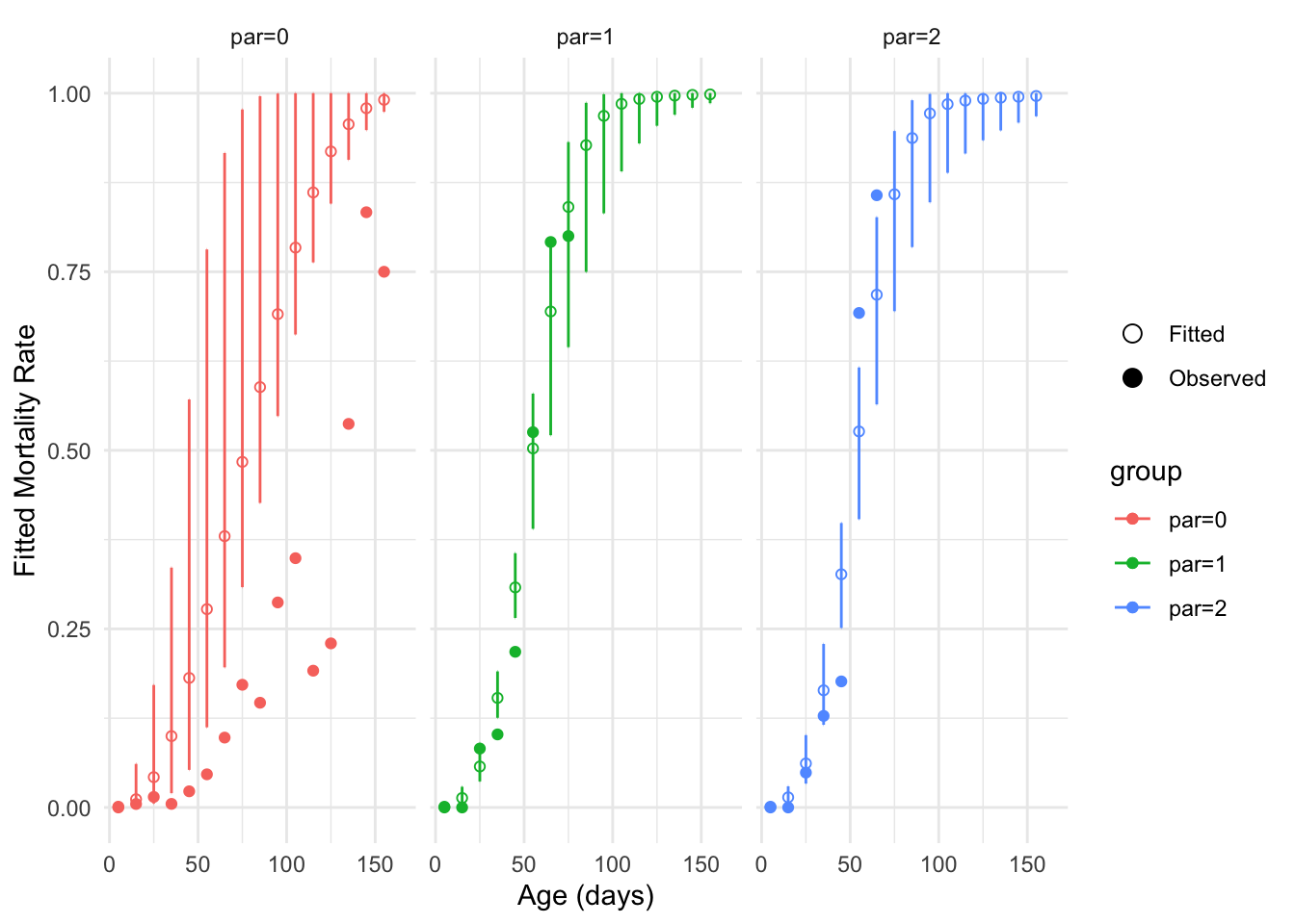
#> maximum bound.Visualization
We can represent the confidence interval computed thanks to the standard errors:
plot_fitted_event_rate(
  results,
  interval_width = 10,
  event = "mortality",
  use_facet = TRUE,
  groupby = "par",
  xlab = "Age (days)",
  ylab = "Fitted Mortality Rate",
  se.fit = TRUE
)
#> Warning: Removed 20 rows containing missing values or values outside the scale range
#> (`geom_point()`).